Practical example/tutorial for MerKurio
This is a brief demonstration and guide on how MerKurio can be used in practice.
Note: this tutorial is written for Unix-like systems.
The guide is also available in the repository, along with the input and output data.
This tutorial assumes that you have already installed MerKurio on your system. If you haven’t done this yet, please refer to the installation section in the documentation. Additionally, the following software is used in this example:
- jq (v1.6)
- Bowtie2 (v2.5.4)
- samtools (v1.22)
- IGV (v2.19.4)
These dependencies are only necessary for parts of the tutorial after read extraction.
In this guide, we will walk through the following scenario: we have a list of relevant k-mers which we have obtained from a fictional association test. We then want to extract all raw sequencing reads from a mutant strain which contain our k-mers of interest, using MerKurio. Next, we want to map them to the wildtype reference genome. With MerKurio, we can then tag the aligned reads with the k-mers they contain and visualize this information in a genome browser.
Setup
To install MerKurio, follow the installation instructions in the Readme or the official documentation.
If you have cargo/Rust installed, you can first clone the repository using git. This will download a local copy of the repository to your computer. Then you can install MerKurio from source, which will automatically add it to your PATH:
git clone https://github.com/lschoenm/MerKurio
cd MerKurio
cargo install --path .
Test the installation by running MerKurio:
merkurio --help
Alternatively, download a standalone binary from the releases page. If you don’t add merkurio to your PATH, you have to call it using the path to the executable.
Download the data
A full dataset of Staphylococcus aureus is available from Zenodo/the Galaxy training network under this link. It comprises the reference genome sequence in FASTA format, a list of feature annotations in GFF format, and paired-end sequence reads in FASTQ format.
First, let’s create a new directory data and download the files by entering the following commands in your terminal:
mkdir data
curl https://zenodo.org/records/582600/files/mutant_R1.fastq > data/mutant_R1.fastq
curl https://zenodo.org/records/582600/files/mutant_R2.fastq > data/mutant_R2.fastq
curl https://zenodo.org/records/582600/files/wildtype.fna > data/wildtype.fna
curl https://zenodo.org/records/582600/files/wildtype.gff > data/wildtype.gff
The dataset contains the following files:
mutant_R[12].fastqare the two FASTQ files containing the paired-end sequencing reads (~150 bp long).wildtype.fnacontains an assembled miniature genome of S. aureus.wildtype.gfflisting the features of the reference genome.
The genome is from an imaginary S. aureus bacterium. The sequencing reads have around 19x coverage.
Extract sequencing reads based on k-mers
Let’s assume that we ran a k-mer-based genome-wide association study in S. aureus which identified the following k-mers to be significantly associated with antibiotics resistance:
AATATAATAAATTAACCGAAGATAAAAAAGAATCTCAGCACATAAATAATGTGGCAGCACAAATTGTGCTGCCACATTATTTATGTGCTGAGA
Normally, we would assume that we already have those sequences obtained from previous analyses either in a text file or a FASTA file - both of which are valid input for MerKurio. For this example, we have to createa file significant_kmers.txt storing these k-mers, one per line. This can be done with the following commands:
echo AATATAATAAATTAACCGAAGATAAAAAAGA > data/significant_kmers.txt
echo ATCTCAGCACATAAATAATGTGGCAGCACAA >> data/significant_kmers.txt
echo ATTGTGCTGCCACATTATTTATGTGCTGAGA >> data/significant_kmers.txt
We can use MerKurio’s extract subcommand to extract all raw sequencing reads from the mutant S. aureus strain which contain any of these k-mers.
The -o flag controls the output file suffix, -i the path to the first input file. We want to extract read pairs if any of the mates contains one of our k-mers. MerKurio automatically switches to paired-end read mode if the second file is provided with the -2 flag.
Because we do not know from which of the two DNA strands the k-mers are coming yet both of them could be represented in the reads, we also have to look for the reverse complements of the query sequences (this is controlled by the -r flag).
Additionally, we would also like to generate detailed match statistics describing which k-mers were found and their exact locations in the reads, along with a few summary statistics. By providing the -l flag without an argument, a log in plain text format is written to the stdout channel of the terminal. Additionally, we can store a log in JSON format by using the -j flag with a file path.
mkdir output
mkdir logs
merkurio extract -i data/mutant_R1.fastq -2 data/mutant_R2.fastq -f data/significant_kmers.txt -r -o output/mutant_extracted -l -j logs/mutant_extracted.stats.json
Here, you can see the statistics log output:
#MerKurio extract log
#2025-06-27T14:54:18+02:00[Europe/Vienna]
#Running merkurio version 1.0.0
#Command line: merkurio extract -i mutant_R1.fastq -2 mutant_R2.fastq -f significant_kmers.txt -r -o mutant_extracted -l -j logs/mutant_extracted.stats.json
#Searching for 6 patterns
#
#File   Record  Pattern Position (zero-based)
mutant_R2.fastq mutant-no_snps.gff-23516/2      ATCTCAGCACATAAATAATGTGGCAGCACAA 30
mutant_R2.fastq mutant-no_snps.gff-23516/2      TCTCAGCACATAAATAATGTGGCAGCACAAT 31
mutant_R2.fastq mutant-no_snps.gff-21992/2      ATTGTGCTGCCACATTATTTATGTGCTGAGA 52
mutant_R2.fastq mutant-no_snps.gff-21992/2      TTGTGCTGCCACATTATTTATGTGCTGAGAT 53
mutant_R2.fastq mutant-no_snps.gff-21086/2      ATCTCAGCACATAAATAATGTGGCAGCACAA 113
mutant_R2.fastq mutant-no_snps.gff-21086/2      TCTCAGCACATAAATAATGTGGCAGCACAAT 114
mutant_R2.fastq mutant-no_snps.gff-21076/2      TCTTTTTTATCTTCGGTTAATTTATTATATT 88
mutant_R2.fastq mutant-no_snps.gff-20088/2      ATCTCAGCACATAAATAATGTGGCAGCACAA 108
mutant_R2.fastq mutant-no_snps.gff-20088/2      TCTCAGCACATAAATAATGTGGCAGCACAAT 109
mutant_R2.fastq mutant-no_snps.gff-18432/2      AATATAATAAATTAACCGAAGATAAAAAAGA 35
mutant_R2.fastq mutant-no_snps.gff-15850/2      TCTTTTTTATCTTCGGTTAATTTATTATATT 29
mutant_R2.fastq mutant-no_snps.gff-14898/2      AATATAATAAATTAACCGAAGATAAAAAAGA 75
mutant_R1.fastq mutant-no_snps.gff-14434/1      TCTTTTTTATCTTCGGTTAATTTATTATATT 66
mutant_R2.fastq mutant-no_snps.gff-13984/2      ATTGTGCTGCCACATTATTTATGTGCTGAGA 113
mutant_R2.fastq mutant-no_snps.gff-13984/2      TTGTGCTGCCACATTATTTATGTGCTGAGAT 114
mutant_R1.fastq mutant-no_snps.gff-12520/1      ATCTCAGCACATAAATAATGTGGCAGCACAA 0
mutant_R1.fastq mutant-no_snps.gff-12520/1      TCTCAGCACATAAATAATGTGGCAGCACAAT 1
mutant_R1.fastq mutant-no_snps.gff-10584/1      AATATAATAAATTAACCGAAGATAAAAAAGA 3
mutant_R1.fastq mutant-no_snps.gff-10384/1      TCTTTTTTATCTTCGGTTAATTTATTATATT 25
mutant_R2.fastq mutant-no_snps.gff-8582/2       ATTGTGCTGCCACATTATTTATGTGCTGAGA 32
mutant_R2.fastq mutant-no_snps.gff-8582/2       TTGTGCTGCCACATTATTTATGTGCTGAGAT 33
mutant_R2.fastq mutant-no_snps.gff-8390/2       TCTTTTTTATCTTCGGTTAATTTATTATATT 14
mutant_R2.fastq mutant-no_snps.gff-7378/2       TCTTTTTTATCTTCGGTTAATTTATTATATT 14
mutant_R2.fastq mutant-no_snps.gff-6398/2       ATTGTGCTGCCACATTATTTATGTGCTGAGA 76
mutant_R2.fastq mutant-no_snps.gff-6398/2       TTGTGCTGCCACATTATTTATGTGCTGAGAT 77
mutant_R1.fastq mutant-no_snps.gff-5520/1       ATCTCAGCACATAAATAATGTGGCAGCACAA 62
mutant_R1.fastq mutant-no_snps.gff-5520/1       TCTCAGCACATAAATAATGTGGCAGCACAAT 63
mutant_R1.fastq mutant-no_snps.gff-5480/1       TCTTTTTTATCTTCGGTTAATTTATTATATT 0
mutant_R2.fastq mutant-no_snps.gff-4756/2       AATATAATAAATTAACCGAAGATAAAAAAGA 113
mutant_R1.fastq mutant-no_snps.gff-3476/1       ATCTCAGCACATAAATAATGTGGCAGCACAA 34
mutant_R1.fastq mutant-no_snps.gff-3476/1       TCTCAGCACATAAATAATGTGGCAGCACAAT 35
mutant_R1.fastq mutant-no_snps.gff-2218/1       TCTTTTTTATCTTCGGTTAATTTATTATATT 51
mutant_R2.fastq mutant-no_snps.gff-2152/2       ATCTCAGCACATAAATAATGTGGCAGCACAA 95
mutant_R2.fastq mutant-no_snps.gff-2152/2       TCTCAGCACATAAATAATGTGGCAGCACAAT 96
mutant_R1.fastq mutant-no_snps.gff-868/1        ATTGTGCTGCCACATTATTTATGTGCTGAGA 8
mutant_R1.fastq mutant-no_snps.gff-868/1        TTGTGCTGCCACATTATTTATGTGCTGAGAT 9
#
#Number of patterns found: 6/6 (100.00 %)
#Pattern        Count
#AATATAATAAATTAACCGAAGATAAAAAAGA        4
#ATCTCAGCACATAAATAATGTGGCAGCACAA        7
#ATTGTGCTGCCACATTATTTATGTGCTGAGA        5
#TCTCAGCACATAAATAATGTGGCAGCACAAT        7
#TCTTTTTTATCTTCGGTTAATTTATTATATT        8
#TTGTGCTGCCACATTATTTATGTGCTGAGAT        5
#
#Total number of records searched: 24960
#Total number of characters searched: 3744000
#Total number of hits: 36
#Number of distinct records with a hit: 24
#
#Total number of hits in file 1: 13
#Total number of hits in file 2: 23
#Number of distinct records with a hit in file 1: 9
#Number of distinct records with a hit in file 2: 15
#Total number of extracted records: 48
Analyzing match statistics
Now we have the extracted sequencing read pairs (those were either mate contained any k-mers) in the files mutant_extracted_1.fastq and mutant_extracted_2.fastq in the output/ directory. Additionally, we have stored the same match statistics that just got printed to the screen in the file mutant_extracted.stats.json in the logs/ folder, but in JSON format instead of plain text. Because it is structured, the JSON file can easily be parsed by other tools or programming languages, making it simple to be used with e.g. Python or R.
A simple yet powerful command-line processor for JSON files is jq. We can use it to inspect the statistics in more detail, for instance to only print the summary statistics:
jq '.summary_statistics' logs/mutant_extracted.stats.json
{
  "number_of_characters_searched": 3744000,
  "number_of_distinct_records_with_a_hit": 24,
  "number_of_matches": 36,
  "number_of_patterns_found": 6,
  "number_of_patterns_searched": 6,
  "number_of_records_searched": 24960
}
If we wanted to do k-mer abundance analysis, we can rank k-mers by frequency:
jq -r '.pattern_hit_counts | to_entries | sort_by(.value) | reverse | .[] | "\(.value)\t\(.key)"' logs/mutant_extracted.stats.json
8	TCTTTTTTATCTTCGGTTAATTTATTATATT
7	TCTCAGCACATAAATAATGTGGCAGCACAAT
7	ATCTCAGCACATAAATAATGTGGCAGCACAA
5	TTGTGCTGCCACATTATTTATGTGCTGAGAT
5	ATTGTGCTGCCACATTATTTATGTGCTGAGA
4	AATATAATAAATTAACCGAAGATAAAAAAGA
Basic calculations are also possible, like calculating the percentage of sequencing reads containing any of our k-mers (note that when extracting read pairs, if at least one mate contains a query k-mer, the number of extracted reads can be higher than the number of matched reads):
jq -r '.summary_statistics | "Extraction rate: \((.number_of_distinct_records_with_a_hit/.number_of_records_searched)*100*1000|round/1000)/100% of reads contained target k-mers"' logs/mutant_extracted.stats.json
Extraction rate: 0.096/100% of reads contained target k-mers
Finally, a more advanced jq command that calculates the hit density per read file, i.e., the average number of matches in extracted sequences, rounded to two decimal places:
jq -r '.paired_end_reads_statistics |
"R1 density: \((.number_of_hits_in_file_1/.number_of_distinct_records_with_a_hit_in_file_1)*100|round/100) hits/read
R2 density: \((.number_of_hits_in_file_2/.number_of_distinct_records_with_a_hit_in_file_2)*100|round/100) hits/read"' \
logs/mutant_extracted.stats.json
R1 density: 1.44 hits/read
R2 density: 1.53 hits/read
Aligning the extracted reads
Now we can map the extracted reads back to the wildtype reference genome, for instance using bowtie2. As a prerequisite, we have to generate an index for our reference:
bowtie2-build data/wildtype.fna data/wildtype
The extracted reads are aligned with the --very-sensitive-local parameter to allow soft-clipping the reads for alignment:
bowtie2 -x data/wildtype -1 output/mutant_extracted_1.fastq -2 output/mutant_extracted_2.fastq --very-sensitive-local > output/mutant_extracted.sam
Tagging the aligned reads with k-mers
It is often a requirement to sort the SAM file by coordinates before doing follow-up analysis. This can be done using samtools:
samtools sort output/mutant_extracted.sam -O sam > output/mutant_extracted.sorted.sam
We would like to know which k-mers the aligned reads contain. To do so, we can use MerKurio’s tag subcommand. Again, we are using the -r flag to also search for reverse complements:
merkurio tag -i output/mutant_extracted.sorted.sam -o output/mutant_extracted.sorted.tagged.sam -f data/significant_kmers.txt -r
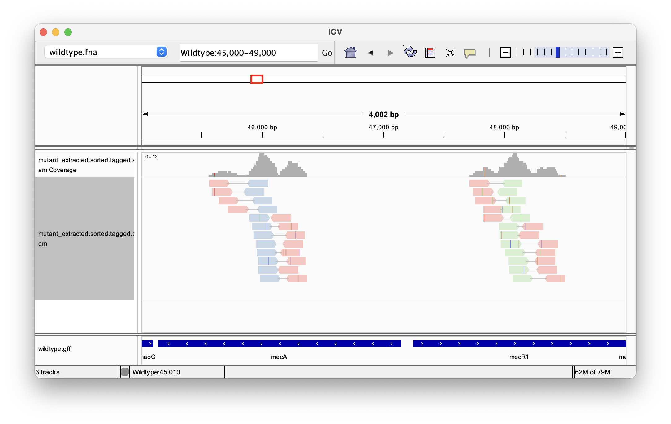
Inspecting the SAM file shows us that the reads are mapped to a region from around 45,000 to 49,000. The k-mers contained in aligned sequences are stored under the km tag (Z denotes a string type, in accordance with the official SAM field specifications):
less output/mutant_extracted.sorted.tagged.sam
Note that we could have also mapped all reads to the reference genome and filter the resulting SAM file to keep only those sequences containing k-mers with merkurio tag -m [...], but in a real-life example with up to terabytes of raw sequencing reads this can become unfeasible, and we would not keep the mates of reads with our k-mers. Extracting only the relevant reads before mapping can save time and disk space.
Visualization of tagged reads
The aligned and tagged sequencing reads can be visualized in the Integrative Genome Browser (IGV). Start IGV (by typing igv in the terminal) and load the wildtype.fna genome, the file with the gene annotations wildtype.gff, and the tagged reads mutant_extracted.sorted.tagged.sam.
To do so, in the menu select “Genomes → Load Genome from File…” and “File → Load from File…”, respectively. IGV might prompt that it must first generate an index for some files.
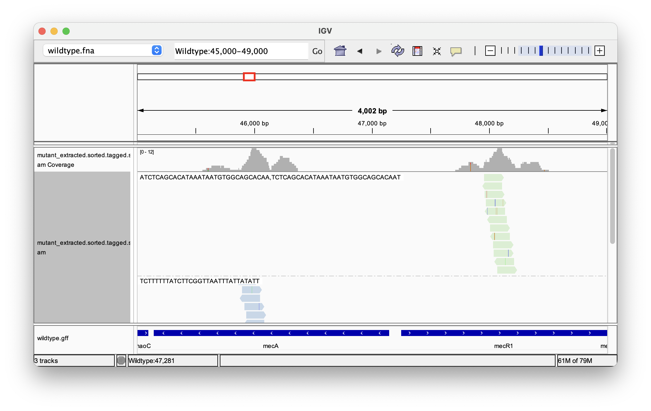
Now, zoom in on the region of interest by entering the coordinates and clicking “Go”: Wildtype:45,000-49,000. Right-clicking on the track with the aligned reads and selecting “View as pairs” to group the read pairs. An advantage of our tagged reads is that we can highlight the presence of specific k-mers. To do so, press right click on the track, go “Color alignments by → tag” and enter km:

Clicking on a single read also shows us its k-mer tags. When looking for specific k-mers, it can also make sense to group them by tag:

By looking at the track with the gene annotations on the bottom, we can see that the reads mapped to positions in the genes mecA and mecR1, which are expressing a penicillin-binding protein and a methicillin-resistance regulatory protein, respectively. By extracting sequencing reads significantly associated with antibiotics resistance and mapping them back to the reference genome we were able to successfully identify candidate genes for this trait.
Follow-up analysis could include looking for variants (SNPs and indels) present in the tagged reads, or intersecting the gene annotation with the positions of extracted reads.